Before actually studying the data mining capabilities of Analysis Services, let us briefly look at some terminology generally used while discussing data mining.
Understanding Terms used in Data Mining
A case is the term used for the facts being studied. The data used to study these facts are called case sets. Each data mining case has a unique identifier called a key. Descriptive pieces of information are called attributes or measures. The case may contain information about a single table or from multiple tables. If there are multiple tables from which data is derived, such a case is defined as a case with nested tables. The hierarchical attributes of a case that can be conveniently grouped are called dimensions of the case.
Clustering breaks down large chunks of data into more manageable groups by identifying similar traits. The clusters provide description of the attributes of the members in each cluster. It is often the first technique that is used in a project and the data is used as a source of future mining efforts as it highlights promising areas to investigate. Microsoft SQL 2000 Analysis Server uses a Scaleable Expectation Maximization algorithm to create clusters based on population density. The advantage of this process is that it requires only a single pass over the entire data and the algorithm creates clusters as it passes and the centers of these clusters are adjusted as more data is processed. It provides reasonable results at any point during its computation. Moreover, it works with a minimum amount of memory.
The strengths of clustering is that it is
1. Undirected
2. Not limited to any type of analysis
3. It handles large case sets
4. Uses minimum memory.
Its weaknesses are:
1. Measurements need to be carefully chosen
2. Results may be difficult to interpret
3. Has no guaranteed value
Another technique used in data mining is the Decision Tree. The Decision tree is used to solve predictive problems. For instance it may be used to predict whether a customer will purchase a particular brand of a product at a particular store in a given geographical location. The algorithm identifies the most relevant characteristics and defines a set of rules that give the percentage of probabilities that new cases will follow the pattern identified.
The decision tree is created using a technique called the recursive partitioning. This algorithm defines the most relevant attributes and splits the population of data on the basis of the attribute. Each partition is called Node. The process is repeated for each subgroup until a good stopping point is found. This may be the point at which all nodes meet the criteria or there are no more nodes that meet the criteria. The last group of cases in the decision tree is called a Leaf node. When all the leaf nodes in a decision tree have only one value the model is said to be over fitted. An over fitted model has the danger of providing unrealistic predictions.
The decision tree model has the following strengths:
1. It provides visual results
2. It is built on understandable rules
3. It is predictive
4. It enables performance for prediction
5. Shows what is important.
On the other hand the weakness of this model is that:
1. It can get spread too thin
2. Performance of training is very expensive as the cases in the node are stored multiple times.
While doing a data mining analysis three distinct types of data sets are used. The initial set of data that is processed and saved for future use is called a training set. This data is used to ‘teach’ the model about the population of data being analyzed. The second set of data required are called test cases. This set is used to build confidence in the hypothesis. Some known attributes are omitted to help us confirm that the model correctly predicts the missing values. The third type of data set used is the evaluation set. The evaluation set focuses on the investigation. It is the final set of cases in which we process the situational data. The model is used to predict behavior based on what the mining activities have learned and is used to drive business strategy.
In the sections that follow we will work on building an OLAP Clustering Data Mining model using the FoodMart 2000 database. We will assume that FoodMart wants to study the loyalty of customers. It will study the number of customers who use FoodMart and how many of them use the FoodMart Club Card. Let us begin by categorizing customer behaviour by using clustering to define the characteristics of people who have the FoodMart Club Card.
The Data mining model can use the OLAP or a Relational Data store. The former allows the user have the advantage of predetermined aggregations and dimensional information from the source cube. The latter requires the user to input information on what describes a complete case. If there are multiple tables the table joins have to be specified.
{mospagebreak}
Creating a Training model and Building Data Mining Model Using OLAP Data store.
In the section here we will build a Data Mining model using OLAP data store.
1. In the Analysis Manager Tree pane expand the FoodMart 2000 database.
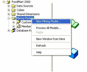
2. Right click on Mining models and select New Mining model… option.
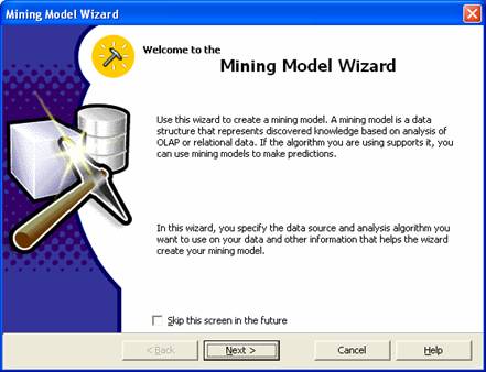
3. The Data mining Wizard opens. Click Next on the Welcome screen to proceed with the creation of the data mining model
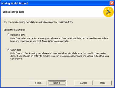
4. The next screen prompts the user select the Data source type. Select OLAP and click Next.
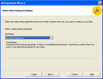
5. Now select the Algorithm for this model. Since we want to use Clustering Algorithm select it and click Next to continue.
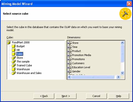
6. Since we are studying customer behavior we will chose the sales cube for our analyses. Click on Sales and click Next
|
|
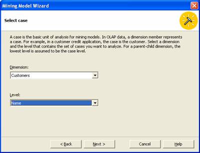
7. By default the lowest level would be store and the level would be Name. We will select Customers as our dimension and Name as the level. Click Next after selecting the above.
|
|
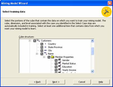
8. The Next step is the selection of the Training data. The Wizard defaults to the selection of the training data from the dimension which was selected in the previous screen. Click Next to continue
|
|
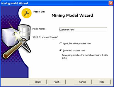
9. Now give the model a name “Customer Sales” and Save and process the model by selecting the appropriate radio button. Click finish to process the mining model.
|
|
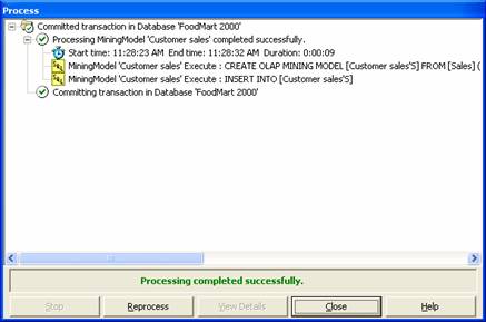
10. The Process log window opens and the Mining model is processed. On successful completion of processing a message is displayed. Close the Process log window. It may be pointed out here that the process log window displays the location where the mining algorithm is being processed. The process can be stopped any time and rebuilt. The user can reprocess the Mining model or simply exit without processing at any time.
|
|
{mospagebreak}
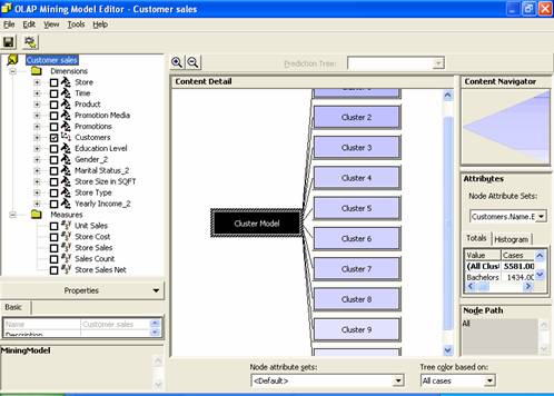
11. The OLAP Mining model Editor opens once the mining model is processed and saved. The model has to be processed before it can be browsed. The data mining model editor displays the results of the analysis. The parameters used to create the cluster are displayed in the left pane. The graphical display is visible in the middle pane and the right pane displays the attributes of the results.
|
|
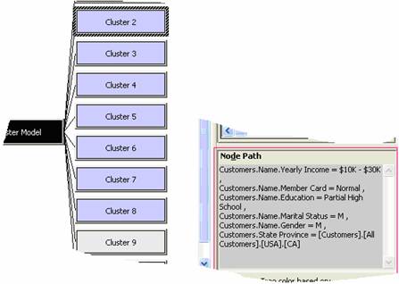
12. On clicking a cluster(in this case Cluster 2) the Node path describes what defines the cluster. By default the attribute set is the first one in the model.
|
|
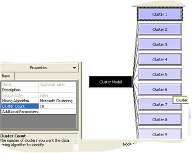
13. The number of clusters generated is by default 10. This can be overridden and the number of clusters to be generated can be increased or decreased to get required results. This is done by clicking on the top node in the left hand pane. The Properties window shows the number of clusters to be generated value. Change the number and reprocess the model for it to take effect.
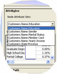
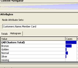
15. Note that there is a bar graph or histogram in the Attributes pane of the Mining model Editor. This gives the values for each of the attributes measured. We can click through the clusters to understand the values of each attribute.
16. As we look, we will realize that the attributes tend to drive the groupings of the model and classify them on the basis of Income, occupation and Education. Now further analysis can be done on the mining model.
|
|
|
[catlist id=181].

