Counting sort is a sorting algorithm that is not based on comparison like most other methods. This method of sorting is used when all elements to be sorted fall in a known, finite and reasonably small range.
How it works:
The algorithm refers to finding for each element a[i] the number of elements from the array that are lower than it.
Step by step example :
Having the following list, let;s try to use counting sort to arrange the numbers from lowest to greatest:
Unsorted list, the array A contains the elements to be sorted:

We count the number of occurrences from the list into the array C, and for example we found one occurrence for the element 3 so far :
PS: A – list of sorting elements, B – Sorted list, C – number of occurences.

The next element is 2, so we increment by 1 the array C and so on until the end of the array:
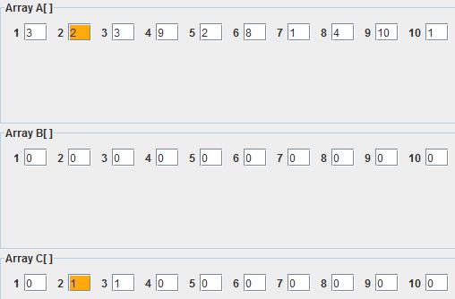
The next element is 3, so we increment by 1 :
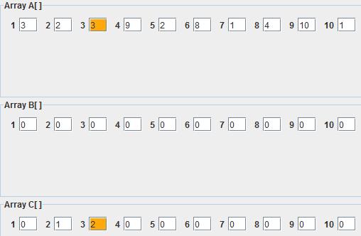
The next element is 9, so we increment by 1 :

The next element is 2, so we increment by 1 :
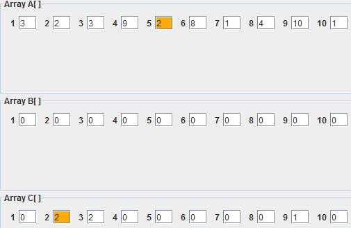
The next element is 8, so we increment by 1 :
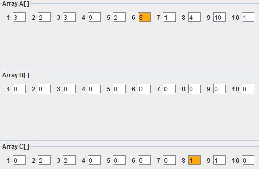
The next element is 1, so we increment by 1 :
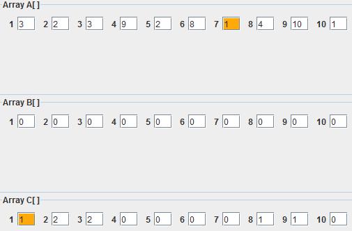
The next element is 4, so we increment by 1 :
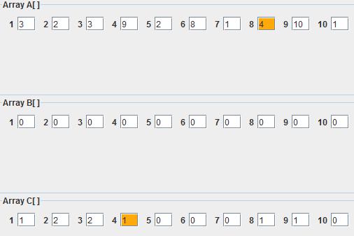
The next element is 10, so we increment by 1 :
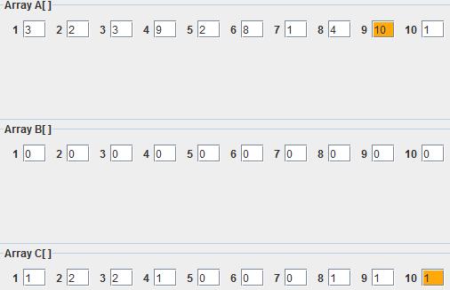
The next element is 1, so we increment by 1 :
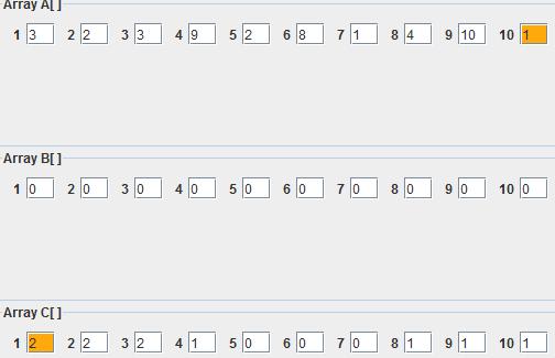
Now, using the elements of the C array, we add the current element with the one from below:
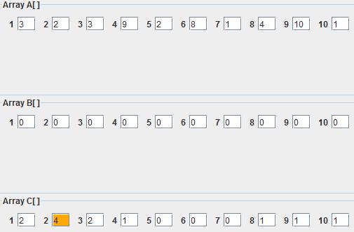
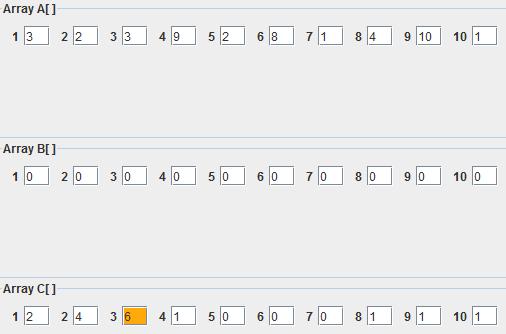

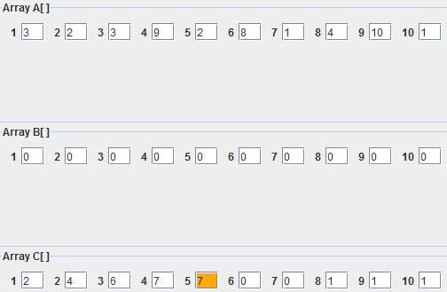
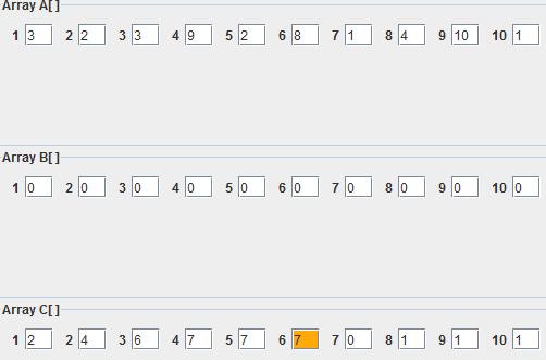

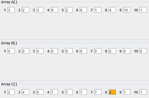
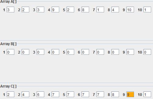

Now let us sort things out a bit. First, look at the last element from the sorting list, which is 1, next look at what number is on the position with 1 as the index from the C array – where all the occurrences are. That number will point to the position in the final sorted array B, which is 2:
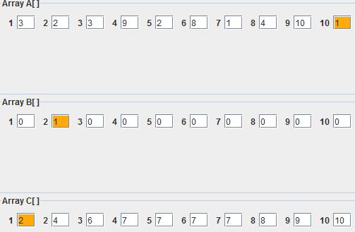
Decrease the number of occurrences by 1 since we found a place for a number:

Now, we do the same for the next element which is 10, and the position for it is 10:
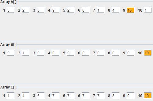
Decrease the number of occurrences by 1 since we found a place for a number:
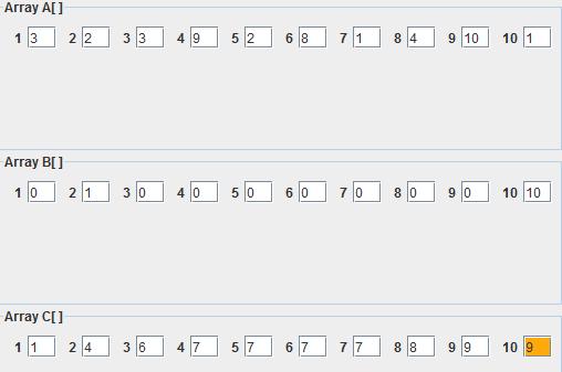
4 is the next element, after which we decrease the number of occurrences:


1 is the next element, after which we decrease the number of occurrences:


8 is the next element, after which we decrease the number of occurrences:

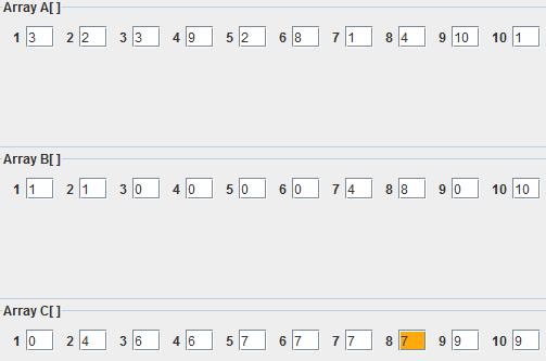
2 is the next element, after which we decrease the number of occurrences:
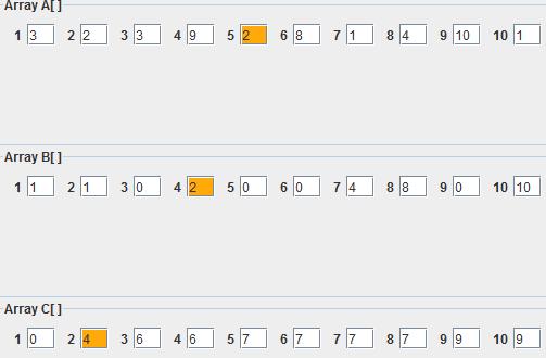

9 is the next element, after which we decrease the number of occurrences:
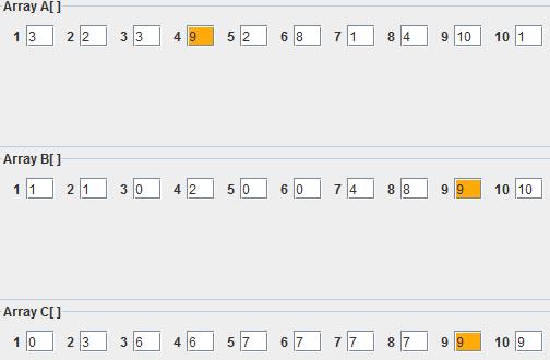

3 is the next element, after which we decrease the number of occurrences:
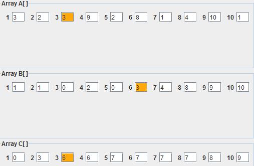
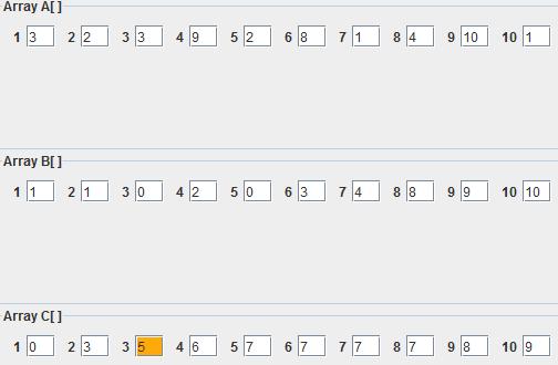
2 is the next element, after which we decrease the number of occurrences:
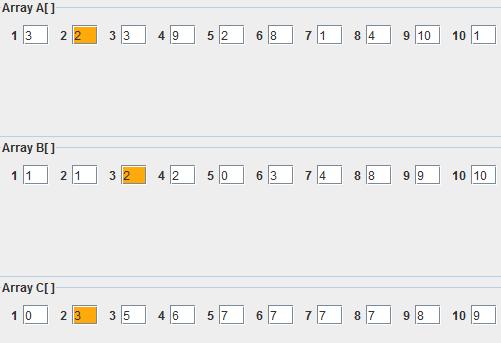

3 is the next element, after which we decrease the number of occurrences:


The data has been sorted! Look at the B array!
Sample code:
#include < iostream >using namespace std;
int main()
{long int A[10000];
long int n = 100;
int *p=new int[50];
int i;
int B[10];
cout << "Please insert the number of elements to be sorted: ";
cin >> n; // The total number of elements
for(int i=0;i< n;i++)
{cout << "Input " << i << " element: ";
cin >>A[i]; // Adding the elements to the array
}cout << "Unsorted list:" << endl; // Displaying the unsorted array
for(int i=0;i < n;i++)
{cout << A[i] << " ";
}int k=A[0];
for(int i=1;i< n;++i)
{if(k< A[i])
{k=A[i];
}}for(int i=0;i< =k;++i)
{p[i]=0;
}for(int j=0;j< n;++j)
{p[A[j]]=p[A[j]]+1;
}for(int i=1;i< =k;++i)
{p[i]=p[i-1]+p[i];
}for(int j=n-1;j>=0;--j)
{i=A[j];
B[p[i]-1]=i;
p[i]=p[i]-1;
}cout << "nSorted list:" << endl; // Displaying the sorted array
for(int i=0;i< n;i++)
{cout << B[i] << " ";
}return 0;
}
Output:

Code explanation:
for(int i=0;i< =k;++i)
{p[i]=0;
}
The array that holds the number of occurrences is p, and at first, all the values will be set to 0.
for(int j=0;j< n;++j)
{p[A[j]]=p[A[j]]+1;
}
The array p is filled up with the number of occurrences for each element.
for(int i=1;i< =k;++i)
{p[i]=p[i-1]+p[i];
}
The sum of the previous element + current element is calculated.
for(int j=n-1;j>=0;--j)
{i=A[j];
B[p[i]-1]=i;
p[i]=p[i]-1;
}
The elements are inserted into the proper places, and the last instruction decrements the number of occurrences.
Complexity:
Counting sort has a running time of O(n + k), where n is the number of elements to be sorted and k is the range of those numbers. If k = O(n), this algorithm has O(n) performance. Counting sort does not sort in place, since it creates two other arrays, counting array C and output array. The space complexity is O(n + k), where n and k are the length of the array A and C, respectively. No swap operations is performed during the process.
Advantages:
- is stable;
- is fast.
Disadvantages:
- unsuitable for strings;
- memory requirement, it requires both an array and a heap of size n;
- not recommended on large sets of data.
Conclusion:
Counting sort may for example be the best algorithm for sorting numbers whose range is between 0 and 100, but it is probably unsuitable for sorting a list of names alphabetically. However, counting sort can be used with radix sort to sort a list of integers whose range is too large for counting sort to be suitable alone.
[catlist id=197].
