Depth-first search (DFS) and breadth-first search (BFS) are two algorithms for traversing a graph. A breadth-first search (BFS) begins at the root node and explores all the neighboring nodes. Then for each of those nearest nodes, it explores their unexplored neighbor nodes, and so on, until it finds the goal.
Example:
In the case of BFS:

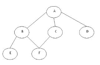
If for DFS the traversal would be A, B, E, F, C, D, in the case of BFS it would be A, B, C, D, E, F. he BFS visits the nodes level by level, so it will start with level 0 which is the root node, and then it moves to the next levels which are B, C and D, then the last levels which are E and F.
Sample code:
#include < iostream >#include < stdlib.h >using namespace std;
int cost[10][10],i,j,k,n,qu[10],front,rare,v,visit[10],visited[10];
int main()
{int m;
cout << "Enter the number of vertices =";
cin >> n;
cout << "Enter number of edges = ";
cin >> m;
cout << "nEDGES n";
for(k=1;k< =m;k++)
{cin >>i>>j;
cost[i][j]=1;
}cout << "Enter initial vertex = ";
cin >>v;
cout << "Visitied verticesn";
cout << v;
visited[v]=1;
k=1;
while(k< n)
{for(j=1;j< =n;j++)
if(cost[v][j]!=0 && visited[j]!=1 && visit[j]!=1)
{visit[j]=1;
qu[rare++]=j;
}v=qu[front++];
cout<< v << " ";
k++;
visit[v]=0; visited[v]=1;
}return 0;
}
Output:

Code explanation:
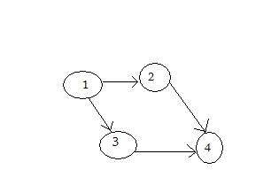
Having the following graph:

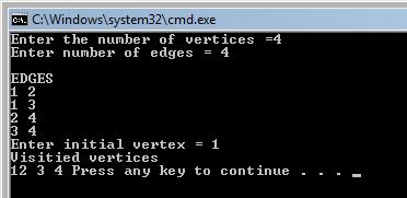
The number of vertices is 4, and the number of edges 4. When inserting the edges, for example we have a edge from 1 to 2, from 1 to 3, from 2 to 4 and for 3 to 4, and if we select the vertex 1 as the starting point, we will get the output from above. The algorithm runs just like in the example from above, it marks the visited vertices, and continues until there is no more vertices to visit.
Complexity:
Time complexity Since in the worst case breadth-first search has to consider all paths to all possible nodes the time complexity of breadth-first search is 1 + b + b^2 + b^3 + … + b^d which is O(b^d). The time complexity can also be expressed as O( | E | + | V | ) since every vertex and every edge will be explored in the worst case.
Applications:
- Maze generation may use a randomized depth-first search.
- Solving puzzles with only one solution, such as mazes. (DFS can be adapted to find all solutions to a maze by only including nodes on the current path in the visited set.)
- Finding 2-(edge or vertex)-connected components.
- Finding connected components.
[catlist id=197].
